This is the second post in a series based off my Python for Data Science bootcamp I run at eBay occasionally. The other posts are:
Jupyter is an interactive computing environment that allows users to create heterogeneous documents called notebooks that can mix executable code, markdown text with MathJax, multimedia, static and interactive charts, and more. A notebook is typically a complete and self-contained record of a computation, and can be converted to various formats and shared with others. Jupyter thus supports a form of literate programming. Several of the posts on this blog, including this one, were written as Jupyter notebooks. Jupyter is an extremely popular tool for doing data science in Python due to its interactive nature, good support for iterative and experimental computation, and ability to create a finished artifact combining both scientific text (with math) and code. It’s easiest to start to understand this by looking at an example of a finished notebook.
Jupyter the application combines three components:
- The notebook application: An front-end interactive application for writing and running code interactively and authoring notebook documents. There are multiple different front-ends available, running on the CLI, natively, or in a browser. The most commonly used front-end is Jupyter Notebook which runs in the browser, although it is due to be replaced by the newer JupyterLab which is currently in beta. As of this writing (April 2018) I recommend using JupyterLab on Mac and Linux but Jupyter Notebook on Windows, as there seem to be some issues still with getting JupyterLab running on Windows.
- Kernels: These are separate processes started by the notebook application that runs the user’s code in a given language and returns output back to the notebook application. The kernel also handles things like computations for interactive widgets, tab completion and introspection. The original kernel was Python and the old version of Jupyter that was for Python only was called IPython; the name was changed to Jupyter to remove the language dependency as kernels exist for a number of different languages now, and IPython is used now to refer to the Python environment for Jupyter. In this overview we are only going to consider that environment.
- Notebook documents: Self-contained documents (JSON text in files with .ipynb extension) that contain a representation of all content visible in the notebook application, including inputs and outputs of the computations, text, images, and more. A notebook can be running which means it is attached to a kernel. Each notebook document has its own kernel.
Notebooks consist of a linear sequence of cells of various types:
- Code cells: live code that is run in the kernel, and the output from running that code
- Markdown cells: text cells formatted with mrkdown with embedded LaTeX (MathJax) equations
- Heading cells: Up to 6 hierarchical levels of header text (I usually don’t use these and just put my headings in markdown cells, but using heading cells can be useful for outline views of a document or table of contents)
- Raw cells: Unformatted text that is included, without modification, when notebooks are converted to different formats using the conversion utility nbconvert
Jupyter documentation is available at https://jupyter-notebook.readthedocs.io/en/stable/
Installing and Running JupyterLab (Mac/Linux)
On Mac and Linux, if you have the Anaconda distribution of Python, install JupyterLab with:
conda install -c conda-forge jupyterlab
or with pip:
pip install jupyterlab
and run with:
jupyter lab
Jupyter Lab will open in a web browser tab displaying a main menu along the top, a file browser on the left listing the notebooks and files in the current directory, and a tabbed interface on the right for open notebooks, terminals, etc.

Running Jupyter Notebook (Windows)
On Windows, use Jupyter Notebook, which is installed as part of the Anaconda distribution, and can be launched directly from Anaconda Navigator or from an Anaconda Python console with:
jupyter notebook
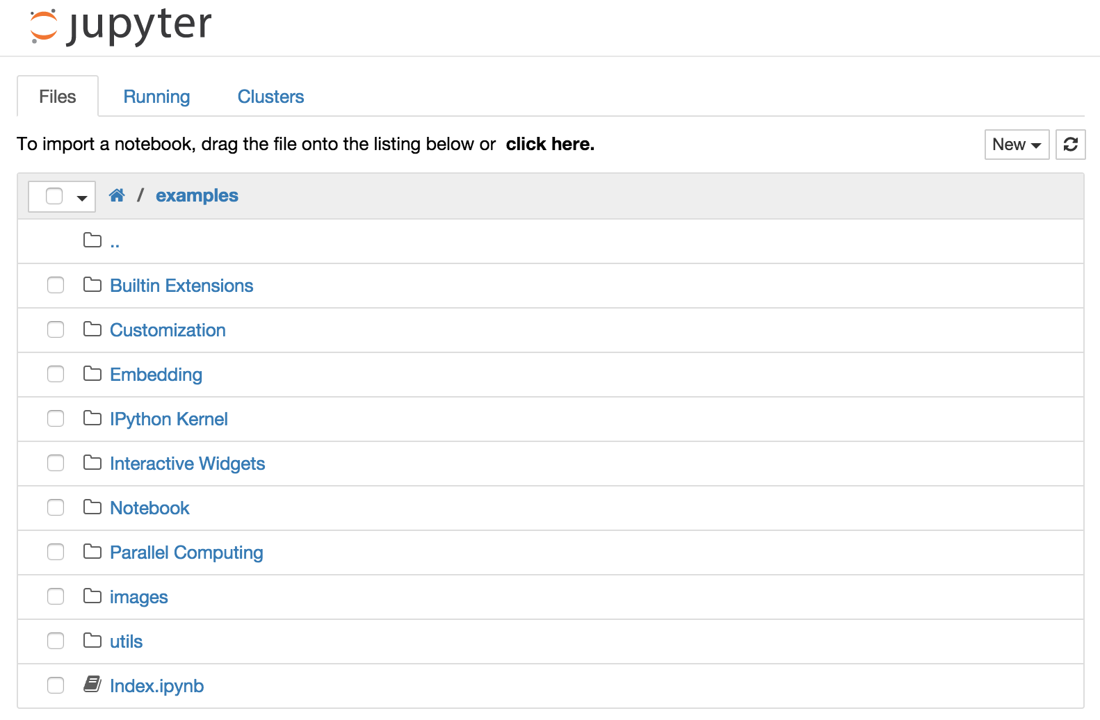
This should open a web browser pointing at the notebook dashboard, which displays the notebooks and files in the current directory.
Jupyter Notebook uses separate browser tabs for each notebook and the filebrowser rather than integrating everything within one browser tab like JupyterLab; nonetheless is should be fairly straightforward to follow along).
Basic Usage
The top of the notebook list displays clickable breadcrumbs of the current directory. By clicking on these breadcrumbs or on sub-directories in the notebook list, you can navigate your file system.
To create a new notebook, use the menu option “File - New - Notebook” (JupyterLab), click on the “New” button at the top of the list and select a kernel from the dropdown menu. Which kernels are listed depend on what’s installed on the server.
The file manager shows a green dot next to running notebooks (as seen below). Notebooks remain running until you explicitly shut them down; closing the notebook’s page is not sufficient.
To view the running notebooks and shutdown a notebook, click the “Running” tab on the left side of the window, and then the “Shutdown” button next to the notebook in question.
To delete, duplicate, or rename a notebook right-click on it in the file browser; a context menu will show with these options along with others.
If you create a new notebook or open an existing one, you will be taken to the notebook user interface within a tab, which allows you to run code and author notebook documents interactively. The notebook UI has a toolbar at the top, followed by the notebook area below, which consists of one or more cells.
The notebook UI is modal. If you click in a cell or press ENTER you enter “edit mode” and can type into the cell. If you click outside a cell or press ESC you will be in “command mode” which allows you to edit the notebook structure.
You can execute a code cell or render a markdown cell by pressing Shift-ESC. Focus will move to the next cell (a new cell will be created if you executed the last cell).
If for some reason your notebook kernel hangs (e.g. waiting on some I/O that never happens, or due to a long running process), you can interrupt the execution by selecting “Interrupt Kernel” from the Kernel menu.
Tutorial
These tutorials are for the old Jupyter Notebook UX, not Jupyter Lab, but are still useful as there is much in common.
Basics: https://jupyter-notebook.readthedocs.io/en/stable/examples/Notebook/Notebook%20Basics.html
http://jakevdp.github.io/blog/2017/03/03/reproducible-data-analysis-in-jupyter/
Markdown
Jupyter supports GitHub-flavored markdown for formatting and styling text in markdown cells; see https://guides.github.com/pdfs/markdown-cheatsheet-online.pdf for a quick reference.
Re-ordering, Inserting, Deleting and Executing Cells
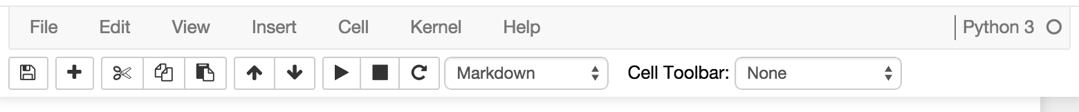
The notebook toolbar, shown above for Jupyter Notebook but similar in Jupyter Lab, has options to save the notebook, add (+), delete (cut) cells, copy cells, paste cells, move cells up or down in the notebook, run the cell, interrupt or restart the kernel, and change the cell type.
To run a cell that has focus, use Shift-Enter. The output of the execution will be added to the notebook. Try it now:
1+2+3+4
10
More generally, you can use Python print statements to print info to the cell output, or you can put a Python expression (often just a variable name) at the end of the code cell and have that print automatically. It’s possible to extend this latter functionality to multiple expressions by executing this code in a cell:
from IPython.core.interactiveshell import InteractiveShell
InteractiveShell.ast_node_interactivity = "all"
or, if you want this to happen automatically every time you start Jupyter, you can edit or create the file ~/.ipython/profile_default/ipython_config.py and add the contents:
c = get_config()

# Run all nodes interactively
c.InteractiveShell.ast_node_interactivity = "all"
If you end the last line with a semi-colon the output will be suppressed:
1+2+3+4;
The result of execution of the most recently executed cell is assigned to a special variable, ‘_’:
print(_)
10
You can put a semicolon at the end of code in a cell to suppress the output:
1+2+3+4;
The cells are labeled with In and Out, and a count. The count allows you to keep track of the order in which cells were executed. Out is the result of execution, unless the execution of the cell resulted in some output to stdout/stderr; in this case that is shown instead with no Out label. Output to stderr is shown in red:
import sys
print('hello', file=sys.stderr)
hello
In and Out are also variables that contain the history of execution (In is a list/array of strings, while Out is a dictionary/hash table):
print(In)
['', '1+2+3+4', '1+2+3+4;', 'print(_)', '1+2+3+4;', "import sys\nprint('hello', file=sys.stderr)", 'print(In)']
print(Out)
{1: 10}
Executing Shell Commands
You can execute a shell command in a cell by starting it with ‘!’. For example, if your notebook relies on certain packages, you may want to start with a cell that uses shell commands to pip install the dependencies.
# On Mac or Linux
!ls -l | head
total 1352
-rw-r--r--  1 gram  staff    4357 Apr 15 10:03 1-1s-hike.md
-rw-r--r--  1 gram  staff  167659 Apr 16 21:16 Python Crash Course.ipynb
-rw-r--r--  1 gram  staff     130 Apr 12 21:07 Python Crash Course.meta
-rw-r--r--  1 gram  staff    2667 Apr 15 10:04 a-christmas-carroll.md
-rw-r--r--  1 gram  staff     585 Apr 11 21:04 accelerated-planning-technique.md
-rw-r--r--  1 gram  staff    3839 Apr 15 10:04 archimedes-counts-the-sand.md
-rw-r--r--  1 gram  staff    2487 Apr 15 10:04 babylonian-numbers-in-60-seconds.md
-rw-r--r--  1 gram  staff    1127 Apr 11 20:50 blogagain.md
-rw-r--r--  1 gram  staff    3569 Apr 15 10:04 capturing-the-elusive-form.md
# On Windows
!dir
It’s possible to assign this to a variable:
# On Mac or Linux
x = !(ls -l | head)
# On Windows
x = !dir
print(x)
['total 1352', '-rw-r--r-- 1 gram staff 4357 Apr 15 10:03 1-1s-hike.md', '-rw-r--r-- 1 gram staff 167659 Apr 16 21:16 Python Crash Course.ipynb', '-rw-r--r-- 1 gram staff 130 Apr 12 21:07 Python Crash Course.meta', '-rw-r--r-- 1 gram staff 2667 Apr 15 10:04 a-christmas-carroll.md', '-rw-r--r-- 1 gram staff 585 Apr 11 21:04 accelerated-planning-technique.md', '-rw-r--r-- 1 gram staff 3839 Apr 15 10:04 archimedes-counts-the-sand.md', '-rw-r--r-- 1 gram staff 2487 Apr 15 10:04 babylonian-numbers-in-60-seconds.md', '-rw-r--r-- 1 gram staff 1127 Apr 11 20:50 blogagain.md', '-rw-r--r-- 1 gram staff 3569 Apr 15 10:04 capturing-the-elusive-form.md']
Checkpoints and Saving
The notebook is saved automatically periodically. Expplicitly saving the notebook from the toolbar or file menu actually creates a time-stamped “checkpoint”, and you can revert to a saved checkpoint from the file menu.
Tips and Tricks
You can write math with MathJax. For example, in a markdown cell, the text:
\\[ P(A \\mid B) = \\frac{P(B \\mid A) \\, P(A)}{P(B)} \\]

Pi is \\(\\pi\\) okay?
will render as shown below when the cell is “executed”:
\[ P(A \mid B) = \frac{P(B \mid A) \, P(A)}{P(B)} \]
Surrounding with single $ signs renders the math inline while double $ renders as a separate block.
You can get help on a Python function (view its docstring) by following it with ? in Jupyter:
import os

os.path.exists?
That requires you to execute the code; you can do the same without executing the whole cell by typing Shift-TAB after the function name. You can also use the built-in Python function help:
help(len)
Help on built-in function len in module builtins:

len(obj, /)
    Return the number of items in a container.
help(os.path.exists)
Help on function exists in module genericpath:

exists(path)
    Test whether a path exists.  Returns False for broken symbolic links
This works on your own functions too so writing docstrings is always recommended.
You can go a step further and use two ?? to get the source code of a function.
import pandas as pd
pd.concat??
Jupyter supports tab-completion with the TAB key (or on every keypress with the hinterland extension; see the section on extensions later to learn how to enable that).
Cell and Line Magics
There are numerous special commands called Ipython Magics that can be used to control things in Jupyter. These are either line magics that start with % or cell magics that start with %%. A line magic consists of a single line, while a cel magic consists of everything from the %% to the end of the cell.
%load can load code from external scripts. We will use that for hiding the answers to some exercises.
%run will let you run an external script or another notebook.
%%time at the start of a cell will time the execution of the cell and print a summary when done. %%timeit will run the code repeatedly (100,000 times by default) and then show the mean of the top 3 times.
%env can be used to set environment variable values.
%%writefile writes the contents of a cell tro a file.
%pycat shows the syntax-highlighted contents of the specirfied Python file in a pop-up window.
%%pdb runs the contents of the cell under control of the Python debugger.
You can use %lsmagic to see all availble magics.
More documentation on magics is available here: http://ipython.readthedocs.io/en/stable/interactive/magics.html
A very common one for data science is %matplotlib inline; this is necessary if using the matplotlib or Seaborn plottting libraries to make sure the plots appear as cell outputs in the notebook. If you have a retina Mac you can use retina-resolution for plots by executing %config InlineBackend.figure_format = 'retina'.
Custom Magics
You can easily create your own magics; they are just Python functions. You just need to import the appropriate Python decorators and then annotate your function. We’re getting ahead of ourselves but a quick example should illustrate:
from IPython.core.magic import register_line_magic

@register_line_magic
def greet(line):
    print(f'Hello {line}!')
%greet Dave
Hello Dave!
Read more here: http://ipython.readthedocs.io/en/stable/config/custommagics.html
The Jupyter Display System
Jupyter can display many different types of output from cells, not just text. This can be determined by the MIME type of the result, but you can use expplicit control too with the IPython.display module:
from IPython.display import display, Image

display(Image('https://www.python.org/static/community_logos/python-logo.png'))

from IPython.display import YouTubeVideo
# a talk about IPython at Sage Days at U. Washington, Seattle.
YouTubeVideo('1j_HxD4iLn8')
Extensions
Jupyter is highly extensible and there are many extensions available. To start using extensions, install the main contributed ones. With conda, run:
conda install -c conda-forge jupyter_contrib_nbextensions
else with pip, run:
pip install jupyter_contrib_nbextensions
Restart Jupyter. In Jupyter Notebook, in the Edit menu you should see a new option nbextensions config. This will open up a new tab where you can easily enable or disable extensions with a checkbox. There doesn’t yet seem to be an equivelent option in JupyterLab for setting these so for now just use Jupyter Notebook for changing which extensions you want enabled.
Going Further
More good tips here: https://www.dataquest.io/blog/jupyter-notebook-tips-tricks-shortcuts/
RISE is an extension that allows you to create a slide deck in Jupyter and present it. Your deck can include live code that you execute, so it is great for Python programming talks :-). See https://github.com/damianavila/RISE for more details.
Here’s an example, which is an overview of Jupyter :-) http://quasiben.github.io/dfwmeetup_2014/#/
For more advanced users, Jupyter can be extended and customized in multiple ways; you can read about them here: https://mindtrove.info/4-ways-to-extend-jupyter-notebook/
Diffing notebooks for use with SCMs like git can be tricky as they are complex JSON files. A tool to help is nbdime: http://nbdime.readthedocs.io/en/stable/
You can find a gallery of interesting notebooks at https://github.com/jupyter/jupyter/wiki/A-gallery-of-interesting-Jupyter-Notebooks
An excellent book on Jupyter is this one by Cyrille Rossant (affiliate link):
